Table of Contents
- Doing tomography, i.e., updating the model based on the sensitivity kernels obtained
- Tomographic full waveform inversion (FWI) / imaging using the sensitivity kernels obtained
- Tomographic tools
- OLD VERSION OF THE SECTION, WILL SOON BE IMPROVED AND ENRICHED
- References
Doing tomography, i.e., updating the model based on the sensitivity kernels obtained
See also the next chapter (Chapter [cha:FWI]) about how to perform full waveform inversion (FWI) or source inversions.
STILL UNDER CONSTRUCTION ... New content will be added soon.
Tomographic full waveform inversion (FWI) / imaging using the sensitivity kernels obtained
One of the fundamental reasons for computing sensitivity kernels (Section [sec:Adjoint-simulation-finite]) is to use them within a tomographic inversion, i.e., perform imaging. In other words, use recorded seismograms, make measurements with synthetic seismograms, and use the misfit between the two to iteratively improve the model described by (at least) $V_{{\rm p}}$, $V_{{\rm s}}$, and $\rho$ as a function of space.
As explained for instance in (Monteiller et al. 2015), full waveform inversion means that one considers the observed seismograms (possibly filtered) as the basic observables that one wants to fit. One thus searches for the model that minimizes the mean squared difference between observed and synthetic seismograms. In other words, the goal is to find a structural model that can explain a larger portion of seismological records, and not simply the phase of a few seismic arrivals.
Whatever misfit function you use for the tomographic inversion (you can find several examples in Tromp, Komatitsch, and Liu (2008) and Tromp, Tape, and Liu (2005)), you will weigh the sensitivity kernels with measurements. Furthermore, you will use as many measurements (stations, components, time windows) as possible per event; hence, we call these composite kernels “event kernels”, which are volumetric fields representing the gradient of the misfit function with respect to one of the variables ($V_{{\rm s}}$). The basic features of an adjoint-based tomographic inversion were illustrated in Tromp, Komatitsch, and Liu (2008) and Tape, Liu, and Tromp (2007) using a conjugate-gradient algorithm. Other, more powerful techniques such as the Limited-Memory Broyden-Fletcher-Goldfarb-Shanno (L-BFGS) method can now be used, as illustrated for instance in (Monteiller et al. 2015).
Principle
We want to minimize the classical waveform misfit function: $$\chi \left( \boldm \right) = \sum_{s=1}^N\sum_{r=1}^M \int_0^T \frac{1}{2} |\boldu(\boldx_r, \boldx_s; t) - \boldd(\boldx_r, \boldx_s; t)| ^{2} \, dt . \label{misfit}$$ This functional quantifies the $L^2$ difference between the observed waveforms $\boldd(\boldx_r, \boldx_s; t)$ at receivers $\boldx_r$, $r = 1, ..., M$ produced by sources at $\boldx_s$, $s=1,...,N$, and the corresponding synthetic seismograms $\boldu(\boldx_r, \boldx_s; t)$ computed in model $\boldm$. While this misfit function is indeed classical, it is worth mentioning that in the case of noisy real data other norms could be used, since in the oil industry for instance it is known that the $L^1$ norm ((Crase et al. 1990; Brossier, Operto, and Virieux 2010)), hybrid $L^1-L^2$ norms ((Bube and Langan 1997)), Hubert norm ((Ha, Chung, and Shin 2009)), Student-t distribution ((Aravkin, Leeuwen, and Herrmann 2011; Jeong et al. 2015)) etc... can be more robust that the $L^2$ norm used here in the context of synthetic data with no noise. In the vicinity of $\boldm$, the misfit function can be expanded into a Taylor series: $$\chi(\boldm+ \delta\boldm) \approx \chi(\boldm)+\boldg(\boldm)\cdot\delta\boldm +\delta\boldm\cdot\mathbf{H}(\boldm)\cdot\delta\boldm \, , \label{local_misfit}$$ where $\boldg(\boldm)$ is the gradient of the waveform misfit function: $$\boldg(\boldm) = \frac{\partial\chi(\boldm)}{\partial\boldm} \, ,$$ and $\mathbf{H}(\boldm)$ the Hessian: $$\mathbf{H}(\boldm) = \frac{\partial^2\chi(\boldm)}{\partial\boldm^2} \, .$$ In the following, for simplicity the dependence of the gradient and Hessian on the model will be implicitly assumed and omitted in the notations. The nearest minimum of $\chi$ in ([local_misfit]) with respect to the model perturbation $\delta \boldm$ is reached for $$\delta \boldm = -\mathbf{H}^{-1} \cdot \boldg \, . \label{Newton}$$ The local minimum of ([misfit]) is thus given by perturbing the model in the direction of the gradient preconditioned by the inverse Hessian.
Computation of the gradient based on the adjoint method
A direct method to compute the gradient is to take the derivative of ([misfit]) with respect to model parameters: $$\frac{\partial\chi(\boldm)}{\partial\boldm} = -\sum_{s=1}^N\sum_{r=1}^M \int_0^T \frac{\partial \boldu(\boldx_r, \boldx_s; t)}{\partial\boldm}\cdot\left[\boldu(\boldx_r, \boldx_s; t) - \boldd(\boldx_r, \boldx_s; t)\right] \, dt \, . \label{calc_gradient}$$ This equation can be reformulated as the matrix-vector product: $$\boldg = -\mathbf{J}^ \cdot \delta \mathbf{d} \, , \label{Jacobian}$$ where $\mathbf{J}^$ is the adjoint of the Jacobian matrix of the forward problem that contains the Fréchet derivatives of the data with respect to model parameters, and $\delta \mathbf{d}$ is the vector that contains the data residuals. The determination of $\mathbf{J}$ would require computing the Fréchet derivatives for each time step in the time window considered and for all the source-station pairs, which is completely prohibitive on current supercomputers (let us note that this situation may change one day). However, it is possible to obtain this gradient without computing the Jacobian matrix explicitly. The approach to determine the gradient without computing the Fréchet derivatives was introduced in nonlinear optimization by (Chavent 1974) working with J. L. Lions, and later applied to seismic exploration problems by (Bamberger, Chavent, and Lailly 1977), (Bamberger et al. 1982), (Lailly 1983) and (Tarantola 1984). The idea is to resort to the adjoint state, which corresponds to the wavefield emitted and back-propagated from the receivers (e.g., Tromp, Tape, and Liu 2005; Tromp, Komatitsch, and Liu 2008; Plessix 2006; Fichtner, Bunge, and Igel 2006).
Let us give an outline of the theory to compute the gradient based on the adjoint method, and refer the reader to e.g. (Tromp, Tape, and Liu 2005) and (Tromp, Komatitsch, and Liu 2008) for further details. The perturbation of the misfit function can be expressed as: $$\delta \chi (\boldm) = \sum_{s=1}^N\sum_{r=1}^M \int_0^T \left[\boldu(\boldx_r, \boldx_s; t) - \boldd(\boldx_r, \boldx_s; t)\right]\cdot \delta \boldu(\boldx_r, \boldx_s; t) \, dt \, , \label{dchi}$$ where $\delta\boldu$ is the perturbation of displacement given by the first-order Born approximation (e.g., Hudson 1977): $$\begin{aligned} \delta \boldu (\boldx_r, \boldx_s; t) & = & -\int_0^t \int_V \left[\delta\rho(\boldx)\mathbf{G}(\boldx_r,\boldx;t-t')\cdot\partial^2_{t'}\boldu(\boldx,\boldx_s;t') \right. \nonumber \ & + & \left. \nabla \mathbf{G}(\boldx_r,\boldx;t-t'):\delta \boldc(\boldx): \nabla\boldu(\boldx;t') \right] \, d^3\boldx \, dt' \, . \label{Born} \end{aligned}$$ In this expression, $\mathbf{G}$ is the Green’s tensor, $\delta\rho$ the perturbation of density, $\delta c$ the perturbation of the fourth-order elasticity tensor, and a colon denotes a double tensor contraction operation. Inserting ([Born]) into ([dchi]) we obtain $$\begin{aligned} \delta \chi (\boldm) & = & -\sum_{s=1}^N\sum_{r=1}^M \int_0^T \left[\boldu(\boldx_r, \boldx_s; t) - \boldd(\boldx_r, \boldx_s; t)\right] \int_0^t \int_V \left[\delta\rho(\boldx)\mathbf{G}(\boldx_r,\boldx;t-t')\cdot\partial^2_{t'}\boldu(\boldx,\boldx_s;t') \right. \nonumber \ & + & \left. \nabla \mathbf{G}(\boldx_r,\boldx;t-t'):\delta \boldc(\boldx):\nabla\boldu(\boldx,t') \right] \, d^3\boldx \, dt' \, dt \,. \end{aligned}$$ Defining the waveform adjoint source for each source $\boldx_s$ $$\boldf^\dagger(\boldx,\boldx_s;t) = \sum_{r=1}^M \left[\boldu(\boldx_r, \boldx_s; T-t) - \boldd(\boldx_r, \boldx_s; T-t)\right] \delta(\boldx-\boldx_r) \, ,$$ and the corresponding adjoint wavefield $$\boldu^\dagger(\boldx,\boldx_s;t) = \int_0^{t'}\int_V\mathbf{G}(\boldx,\boldx';t'-t)\cdot\boldf^\dagger(\boldx',\boldx_s;t)\, d^3\boldx' \, dt \, ,$$ the perturbation of the misfit function may be expressed as: $$\begin{aligned} \delta\chi(\boldm) & = & - \sum_{s=1}^N\nonumber \int_V \int_0^T \left[\delta\rho \, \boldu^\dagger(\boldx,\boldx_s;T-t)\cdot \partial^2_{t}\boldu(\boldx,\boldx_s;t) \right. \nonumber \ & + & \left. \nabla\boldu^\dagger(\boldx,\boldx_s;T-t):\delta \boldc: \nabla \boldu(\boldx,\boldx_s;t) \right] \, d^3\boldx \, dt \, . \label{dchi2} \end{aligned}$$ At this point, we make some assumptions on the nature of the elasticity tensor. A general fourth-order elasticity tensor is described by 21 elastic parameters, a very large number that makes its complete characterization way beyond the reach of any tomographic approach. For the time being, let us thus consider isotropic elasticity tensors, described by the two Lamé parameters $\lambda$ and $\mu$: $$c_{ijkl} = \lambda \delta_{ij}\delta_{kl}+\mu(\delta_{ik}\delta_{jl}+\delta_{il}\delta_{jk}) \, .$$ In this case, ([dchi2]) can be written as: $$\begin{aligned} \delta\chi(\boldm) & = & - \sum_{s=1}^N\nonumber \int_V \left[ K_\rho(\boldx,\boldx_s)\delta\ln\rho(\boldx) +K_\lambda(\boldx,\boldx_s)\delta\ln\lambda(\boldx) \right. \nonumber \ & + & \left. K_\mu(\boldx,\boldx_s)\delta\ln\mu(\boldx)\right] \, d^3\boldx \, , \label{dchi2_1} \end{aligned}$$ where ln() is the natural logarithm and where the Fréchet derivatives with respect to the density and Lamé parameters are given by: $$\begin{aligned} K_\rho(\boldx,\boldx_s) & = & - \int_0^T \rho(\boldx) \boldu^\dagger(\boldx,\boldx_s;T-t)\cdot \partial^2_{t}\boldu(\boldx,\boldx_s;t) \, dt \ K_\lambda(\boldx,\boldx_s) & = & - \int_0^T \lambda(\boldx) \nabla\cdot\boldu^\dagger(\boldx,\boldx_s;T-t) \nabla\cdot\boldu(\boldx,\boldx_s;t) \, dt \ K_\mu(\boldx,\boldx_s) & = & -2 \int_0^T \mu(\boldx) (\boldx) \nabla\boldu^\dagger(\boldx,\boldx_s;T-t) :\nabla\boldu(\boldx,\boldx_s;t)\, dt \, . \end{aligned}$$ Since the propagation of seismic waves mainly depends on compressional wave speed $\alpha$ and shear wave speed $\beta$, but also because these seismic velocities are easier to interpret, tomographic models are usually described based on these two parameters. With this new parametrization, the perturbation of the misfit function may be written as: $$\begin{aligned} \delta\chi(\boldm) & = & - \sum_{s=1}^N\nonumber \int_V \left[ K'\rho(\boldx,\boldx_s)\delta\ln\rho(\boldx) +K'\alpha(\boldx,\boldx_s)\delta\ln\alpha(\boldx) \right. \nonumber \ & + & \left. K'\beta(\boldx,\boldx_s)\delta\ln\beta(\boldx)\right] \, d^3\boldx \, , \end{aligned}$$ where $$\begin{aligned} K'\rho(\boldx,\boldx_s) & = & K_\rho(\boldx,\boldx_s)+K_\lambda(\boldx,\boldx_s)+K_\mu(\boldx,\boldx_s) \ K'\alpha(\boldx,\boldx_s) & = & 2 \left(\frac{\lambda+2\mu}{\lambda}\right) K\lambda(\boldx,\boldx_s) \ K'\beta(\boldx,\boldx_s) & = & 2 K\mu -\frac{4\mu}{\lambda} K_\lambda (\boldx,\boldx_s) \, . \end{aligned}$$
As can be seen from these expressions, the principle of the adjoint-state method is to correlate two wavefields: the direct (i.e. forward) field that propagates from the source to the receivers, and the adjoint field that propagates from all the receivers backward in time. The same approach can be followed for any type of seismic observable (phase, amplitude, envelope, time series...), provided the appropriate adjoint source is used (Tromp, Tape, and Liu 2005; Tromp, Komatitsch, and Liu 2008). For example, for the cross-correlated traveltime of a seismic phase, the adjoint source is defined as the velocity of that synthetic phase weighted by the travel-time residual.
Computing the gradient based on the adjoint-state method requires performing two simulations per source (forward and adjoint fields) regardless of the type of observable. However, to define the adjoint field one must know the adjoint source, and that source is computed from the results of the forward simulation. One must therefore perform the forward simulation before the adjoint simulation. A straightforward solution for time-domain methods would be to store the whole forward field to disk at each time step during the forward run and then read it back during the adjoint simulation to calculate the interaction of these two fields. In 2-D this is feasible but in the 3-D case for very short seismic periods and without lossy compression, downsampling, or a large amount of disk or memory checkpointing (e.g., Fichtner et al. 2009; Rubio Dalmau et al. 2014; Cyr, Shadid, and Wildey 2015) the amount of disk storage required would currently be too large.
However let us note again that this situation will change in the future. In the mean time, a standard possible solution is to perform three simulations per source (Tromp, Komatitsch, and Liu 2008; Peter et al. 2011), i.e., perform the forward calculation twice, once to compute the adjoint sources and once again at the same time as the adjoint simulation to correlate the two fields and sum their interaction on the fly over all the time steps. Doing so for an elastic Earth, one only needs a small amount of disk storage to store the last time step of the forward run, which is then used as an initial condition to redo the forward run backwards, as well as the field on the outer edges of the mesh for each time steps in order to be able to undo the absorbing boundary conditions.
Tomographic tools
Besides the ability to compute adjoint sensitivity kernels, the SPECFEM3D package provides a number of tools useful for post-processing kernels, gradients and conducting tomographic model updates. The tomographic and post-processing tools can be compiled by typing in the main directory:
make tomography
make postprocess
You can modify specific settings affecting, e.g., the (isotropic) parameterization or directory setup structure in file setup/constants_tomography.h. The compiled binaries can be found in directory bin/.
The iterative inversion workflow may comprise three main steps for which tools are provided:
-
Summing event kernels, e.g. $K_{\alpha,\beta,\rho}$, to build the misfit gradient $\boldg(\boldm)$
-
Smoothing and post-processing of the gradient $\boldg(\boldm)$
-
Updating the model $\boldm_{i+1} = \boldm_i + \delta\boldm$.
Please note that the tomographic routines are very similar for both SPECFEM3D_Cartesian and SPECFEM3D_GLOBE versions. Some differences occur, e.g., when reading in mesh files and when the maximum of the gradient is taken for the update step length. Also note that currently only the binary database format is supported, no ADIOS file format support is implemented yet. In future, we plan to extend and merge these into the same set of tools within a common SPECFEM function library.
Summing kernels
For summing different event kernels, the executables xsum_kernels and xsum_preconditioned_kernels can be used. The binaries sum up either a set of isotropic or transversely isotropic kernel files, depending on the setting in file setup/constants_tomography.h. The following parameterizations can be chosen:
-
isotropic kernels $K_{\alpha,\beta,\rho}$ or
-
isotropic bulk kernels $K_{c,\beta,\rho}$, or
-
transversely isotropic bulk kernels $K_{c,\beta_v,\beta_h,\eta}$.
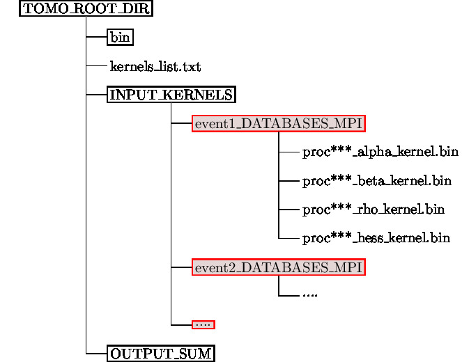
The tools for summing event kernels can be used in parallel, using the same number of processes (NPROC) as the forward/kernel simulations. The summation tools use the following input/output format (see Fig. 1.1 for the default directory structure):
-
Input: Input is provided by a list of event directories, given in file
kernels_list.txt(default setting forKERNEL_FILE_LISTinconstants_tomography.h). The file lists all event kernel directories which should be summed together. All event directories have to be located in directoryINPUT_KERNELS/, which can be setup as links to all individual event kernel directories. -
Output: The summed kernels will be stored in corresponding kernel files in output directory
OUTPUT_SUM/.
Kernel summation:
As example with a total of 4 MPI processes
mpirun -np 4 ./bin/xsum_kernels
adds sensitivity kernels $K$ from different events together, i.e. outputs $\boldg$ where $$\boldg = \Sum^{N}_i K^{i} \nonumber$$ for events $i = 1,..,N$ as specified in file kernel_list.txt.
Kernel Summation with Preconditioning:
As example with a total of 4 MPI processes
mpirun -np 4 ./bin/xsum_preconditioned_kernels
adds sensitivity kernels $K$ together from different events and "preconditions" the sum by dividing with the sum of the corresponding approximate Hessians $\tilde{H}$, i.e. outputs $\boldg$ where $$\boldg = \frac{1}{\Sum_i \tilde{H}^{i}} \; \Sum_i K^{i} \nonumber$$ In this case, the factor $\frac{1}{\Sum_i \tilde{H}^{i}}$ acts as preconditioner, approximating the inverse of the Hessian $\mathbf{H}^{-1}$.
Kernel names: The summation tool will look for kernels with following names:
- for an isotropic model parameterization, kernel names are:
[TABLE]
- for an isotropic bulk model parameterization, kernel names are:
[TABLE]
- for a transversely isotropic model parameterization, kernel names are:
[TABLE]
Note that these event kernels are stored after a kernel simulation (SIMULATION_TYPE = 3) in the LOCAL_PATH directory, which by default points to directory DATABASES_MPI/. Isotropic kernels will be created by default. To create transversely isotropic kernels, you set ANISOTROPIC_KL and SAVE_TRANSVERSE_KL to .true. in the parameter file DATA/Par_file.
- for preconditioning, the approximate Hessian kernels taken for summation are:
[TABLE]
These Hessian kernels approximate the diagonal elements of the Hessian matrix and can be used as preconditioner in a gradient optimization scheme. To create these kernels, you have to set APPROXIMATE_HESS_KL to .true. in the parameter file DATA/Par_file.
For SPECFEM3D_GLOBE, by default only kernels in the crust/mantle region ("reg1") will be considered for summation. You can change the default by setting parameter REG in file constants_tomography.h to the region of interest.
Note that although we provide the preconditioned summation here, we recommend to smooth first both, the summed kernels and summed approximate Hessians, before inverting the summed Hessian and applying it as preconditioner to the gradient. From experience, we prefer doing $$\boldg = \frac{1}{\mathcal{F}{smooth} \left( \Sum^{N}_i \tilde{H}^{i} \right) } \; \mathcal{F}{smooth} \left( \Sum_i K^{i} \right) \nonumber$$ rather than $$\boldg = \mathcal{F}_{smooth} \left( \frac{1}{\Sum^{N}_i \tilde{H}^{i}} \; \Sum_i K^{i} \right) \: . \nonumber$$ Due to the large sensitivity kernel values close to source and receiver locations, the inverse of the thresholded summed Hessian becomes better balanced in the former.
Smoothing and post-processing
For additional smoothing and post-processing of kernels, gradients, or models, we provide tools useful for gradient and model preparation. These additional tools for post-processing sensitivity kernels are provided together with the main package. For compilation of these tools, you type in the main directory:
make postprocess
The following tools are provided:
-
xsmooth_semis used for smoothing with a gaussian function. -
xclip_semis used to threshold a kernel, gradient or model, clipping to a minimum and maximum value. -
xcombine_semis used to combine different event kernels, gradient or model files, summing all individually specified files together (similar toxsum_kernelsbut more flexible).
The post-processing tools are primarily intented to be used to process kernel files. They can be used though on any scalar field of dimension (NGLLX,NGLLY,NGLLZ,NSPEC). The tools are parallel programs – they must be invoked with mpirun or other appropriate utility. Operations are performed in embarrassingly-parallel fashion.
Smoothing:
To smooth a kernel, gradient or model file, use
mpirun -np NPROC bin/xsmooth_sem SIGMA_H SIGMA_V KERNEL_NAME INPUT_DIR OUPUT_DIR
with command line arguments: SIGMA_H horizontal smoothing radius, SIGMA_V vertical smoothing radius, KERNEL_NAME kernel name, e.g. alpha_kernel, INPUT_DIR directory from which kernels are read, OUTPUT_DIR directory to which smoothed kernels are written.
This smooths kernels by convolution with a Gaussian, and writes the resulting smoothed kernels to OUTPUT_DIR.
Files written to OUTPUT_DIR have the suffix ’smooth’ appended, e.g. proc***alpha_kernel.bin becomes proc***alpha_kernel_smooth.bin.
Clipping:
Values in a kernel, gradient or model binary file can be clipped with a minimum/maximum threshold value using
mpirun -np NPROC bin/xclip_sem MIN_VAL MAX_VAL KERNEL_NAMES INPUT_FILE OUTPUT_DIR
with command line arguments: MIN_VAL threshold below which array values are clipped, MAX_VAL threshold above which array values are clipped, KERNEL_NAMES one or more kernel names separated by commas, INPUT_DIR directory from which arrays are read, OUTPUT_DIR directory to which clipped array are written.
For each name in KERNEL_NAMES, reads kernels from INPUT_DIR, applies thresholds, and writes the resulting clipped kernels to OUTPUT_DIR.
KERNEL_NAMES is a comma-delimited list of kernel names, e.g. alphav_kernel,alphah_kernel.
-
For example, in this case type
mpirun -np 4 ./bin/xclip_sem -0.1 0.1 alphav_kernel,alphah_kernel DIR1/ DIR1/
to clip the corresponding kernels in directory DIR1 to be in range $[-0.1,0.1]$.
Files written to OUTPUT_DIR have the suffix ’clip’ appended, e.g. proc***alpha_kernel.bin becomes proc***alpha_kernel_clip.bin
Combining:
To combine kernel values from different kernel directories, you can use
mpirun -np NPROC bin/xcombine_sem KERNEL_NAMES INPUT_FILE OUTPUT_DIR
with command line arguments: KERNEL_NAMES one or more kernel names separated by commas, INPUT_FILE text file containing list of kernel directories, OUTPUT_PATH directory to which summed kernels are written.
For each name in KERNEL_NAMES, sums kernels from directories specified in INPUT_FILE. Writes the resulting sums to OUTPUT_DIR.
INPUT_FILE is a text file containing a list of absolute or relative paths to kernel directories, one directory per line.
KERNEL_NAMES is a comma-delimited list of kernel names, e.g. alpha_kernel,beta_kernel,rho_kernel.
Model updating
We provide (simple) tools for updating the current model $\boldm_i$ using a gradient $\boldg$ and steplength $\alpha$:, i.e. $$\boldm_{i+i} = \boldm_i + \delta \boldm \nonumber$$ with $$\delta \boldm = - \alpha \, \boldg \nonumber \: .$$ The following tomographic tools are provided:
xadd_model_isocan be used to update isotropic model files with a (summed & smoothed) gradient. The gradient files are given for isotropic parameters or isotropic bulk parameters.
Note that instead of using the density kernels $K_{\rho}$ for model updates, setting USE_RHO_SCALING to .true. will ignore the density kernel and use density perturbations scaled from isotropic $V_s$ pertubations.
Isotropic model update:
The program xadd_model_iso can be used to update isotropic model files with (smoothed & summed) event kernels:
mpirun -np 4 bin/xadd_model_iso step_factor [INPUT-KERNELS-DIR/] [OUTPUT-MODEL-DIR/]
with command line arguments: step_factor the step length to scale the gradient, e.g. $0.03$ for a $\pm 3$% update, INPUT-KERNELS-DIR/ (optional) directory which holds summed kernels (e.g. proc***alpha_kernel.bin,.., by default directory INPUT_GRADIENT/ is used), OUTPUT-MODEL-DIR/ (optional) directory which will hold new model files (e.g. proc***vp_new.bin,.., by default directory OUTPUT_MODEL/ is used).
The gradients are given for isotropic parameters (alpha,beta,rho) or (bulk_c,beta,rho).
The algorithm uses a steepest descent method with a step length determined by the given maximum update percentage.
By default, the directory and file setup used is:
-
directory
INPUT_MODEL/contains:proc_vs.bin proc_vp.bin proc***_rho.bin
-
directory
INPUT_GRADIENT/contains:proc_bulk_c_kernel_smooth.bin proc_bulk_beta_kernel_smooth.bin proc***_rho_kernel_smooth.bin
or
  proc***_alpha_kernel_smooth.bin
  proc***_beta_kernel_smooth.bin
  proc***_rho_kernel_smooth.bin
depending on the model parameterization.
-
directory
topo/contains:proc***_external_mesh.bin
for the Cartesian version, and
proc***_solver_data.bin
for the GLOBE version.
The new model files are stored in directory OUTPUT_MODEL/ as
proc***_vp_new.bin
proc***_vs_new.bin
proc***_rho_new.bin
Note that additional post-processing and model update tools are provided for the SPECFEM3D_GLOBE version and will be provided for the Cartesian version as well in future.
OLD VERSION OF THE SECTION, WILL SOON BE IMPROVED AND ENRICHED
There are many other versions of gradient-based inversion algorithms that could alternatively be used (see e.g. (Virieux and Operto 2009; Monteiller et al. 2015) for a list). The tomographic inversion of Tape et al. (2009, 2010) used SPECFEM3D_Cartesian as well as several additional components which are also stored on the CIG svn server, described next.
The directory containing external utilities for tomographic inversion using SPECFEM3D Cartesian (or other packages that evaluate misfit functions and gradients) is in directory utils/ADJOINT_TOMOGRAPHY_TOOLS/:
flexwin/     -- FLEXWIN algorithm for automated picking of time windows
measure_adj/ -- reads FLEXWIN output file and makes measurements,
                with the option for computing adjoint sources
iterate_adj/ -- various tools for iterative inversion
                (requires pre-computed "event kernels")
This directory also contains a brief README file indicating the role of the three subdirectories, flexwin (Maggi et al. 2009), measure_adj, and iterate_adj. The components for making the model update are there; however, there are no explicit rules for computing the model update, just as with any optimization problem. There are options for computing a conjugate gradient step, as well as a source subspace projection step.
The best single file to read is probably: ADJOINT_TOMO/iterate_adj/cluster/README.
References
Aravkin, Aleksandr, Tristan van Leeuwen, and Felix Herrmann. 2011. “Robust Full-Waveform Inversion Using the Student’s $t$-Distribution.” In SEG Technical Program Expanded Abstracts 2011, 2669–73. https://doi.org/10.1190/1.3627747.
Bamberger, A., G. Chavent, Ch. Hemons, and P. Lailly. 1982. “Inversion of Normal Incidence Seismograms.” Geophysics 47 (5): 757–70.
Bamberger, A., G. Chavent, and P. Lailly. 1977. “Une Application de La Théorie Du Contrôle à Un Problème Inverse de Sismique.” Annales de Géophysique 33 (1/2): 183–200.
Brossier, R., S. Operto, and J. Virieux. 2010. “Which Data Residual Norm for Robust Elastic Frequency-Domain Full Waveform Inversion?” Geophysics 75 (3): R37–46.
Bube, Kenneth P., and Robert T. Langan. 1997. “Hybrid $L^1/L^2$ Minimization with Applications to Tomography.” Geophysics 62 (4): 1183–95. https://doi.org/10.1190/1.1444219.
Chavent, G. 1974. “Identification of Function Parameters in Partial Differential Equations.” In Identification of Parameter Distributed Systems, edited by R. E. Goodson and M. Polis, 31–48. American Society of Mechanical Engineers.
Crase, E., A. Pica, M. Noble, J. McDonald, and A. Tarantola. 1990. “Robust Elastic Non-Linear Waveform Inversion: Application to Real Data.” Geophysics 55: 527–38.
Cyr, E. C., J. N. Shadid, and T. Wildey. 2015. “Towards Efficient Backward-in-Time Adjoint Computations Using Data Compression Techniques.” Comput. Methods Appl. Mech. Eng. 288: 24–44. https://doi.org/10.1016/j.cma.2014.12.001.
Fichtner, A., H.-P. Bunge, and H. Igel. 2006. “The Adjoint Method in Seismology: I. Theory.” Phys. Earth Planet. Inter. 157 (1-2): 86–104. https://doi.org/10.1016/j.pepi.2006.03.016.
Fichtner, A., B. L. N. Kennett, H. Igel, and H. P. Bunge. 2009. “Full Seismic Waveform Tomography for Upper-Mantle Structure in the Australasian Region Using Adjoint Methods.” Geophys. J. Int. 179 (3): 1703–25.
Ha, Taeyoung, Wookeen Chung, and Changsoo Shin. 2009. “Waveform Inversion Using a Back-Propagation Algorithm and a Huber Function Norm.” Geophysics 74 (3): R15–24. https://doi.org/10.1190/1.3112572.
Hudson, J. A. 1977. “Scattered Waves in the Coda of $P$.” J. Geophys. Res. 43: 359–74.
Jeong, Woodon, Minji Kang, Shinwoong Kim, Dong-Joo Min, and Won-Ki Kim. 2015. “Full Waveform Inversion Using Student’s $t$ Distribution: A Numerical Study for Elastic Waveform Inversion and Simultaneous-Source Method.” Pure Appl. Geophys. 172 (6): 1491–1509. https://doi.org/10.1007/s00024-014-1020-7.
Lailly, P. 1983. “The Seismic Inverse Problem as a Sequence of Before-Stack Migrations.” In Proceedings of the Conference on Inverse Scattering, Theory and Application Expanded Abstracts, edited by J. B. Bednar, R. Redner, E. Robinson, and A. Weglein, 206–20. Philadelphia, PA, USA: Society of Industrial; Applied Mathematics.
Maggi, A., C. Tape, M. Chen, D. Chao, and J. Tromp. 2009. “An Automated Time-Window Selection Algorithm for Seismic Tomography.” Geophys. J. Int. 178: 257–81.
Monteiller, Vadim, Sébastien Chevrot, Dimitri Komatitsch, and Yi Wang. 2015. “Three-Dimensional Full Waveform Inversion of Short-Period Teleseismic Wavefields Based Upon the SEM-DSM Hybrid Method.” Geophys. J. Int. 202 (2): 811–27. https://doi.org/10.1093/gji/ggv189.
Peter, Daniel, Dimitri Komatitsch, Yang Luo, Roland Martin, Nicolas Le Goff, Emanuele Casarotti, Pieyre Le Loher, et al. 2011. “Forward and Adjoint Simulations of Seismic Wave Propagation on Fully Unstructured Hexahedral Meshes.” Geophys. J. Int. 186 (2): 721–39. https://doi.org/10.1111/j.1365-246X.2011.05044.x.
Plessix, R. E. 2006. “A Review of the Adjoint-State Method for Computing the Gradient of a Functional with Geophysical Applications.” Geophys. J. Int. 167 (2): 495–503.
Rubio Dalmau, F., M. Hanzich, J. de la Puente, and N. Gutiérrez. 2014. “Lossy Data Compression with DCT Transforms.” In Proceedings of the EAGE Workshop on High Performance Computing for Upstream, HPC30. Chania, Crete, Greece. https://doi.org/10.3997/2214-4609.20141939.
Tape, Carl, Qinya Liu, Alessia Maggi, and Jeroen Tromp. 2009. “Adjoint Tomography of the Southern California Crust.” Science 325: 988–92.
———. 2010. “Seismic Tomography of the Southern California Crust Based on Spectral-Element and Adjoint Methods.” Geophys. J. Int. 180: 433–62.
Tape, Carl, Qinya Liu, and Jeroen Tromp. 2007. “Finite-Frequency Tomography Using Adjoint Methods - Methodology and Examples Using Membrane Surface Waves.” Geophys. J. Int. 168 (3): 1105–29. https://doi.org/10.1111/j.1365-246X.2006.03191.x.
Tarantola, A. 1984. “Inversion of Seismic Reflection Data in the Acoustic Approximation.” Geophysics 49: 1259–66.
Tromp, Jeroen, Dimitri Komatitsch, and Qinya Liu. 2008. “Spectral-Element and Adjoint Methods in Seismology.” Communications in Computational Physics 3 (1): 1–32.
Tromp, Jeroen, Carl Tape, and Qinya Liu. 2005. “Seismic Tomography, Adjoint Methods, Time Reversal and Banana-Doughnut Kernels.” Geophys. J. Int. 160 (1): 195–216. https://doi.org/10.1111/j.1365-246X.2004.02453.x.
Virieux, J., and S. Operto. 2009. “An Overview of Full-Waveform Inversion in Exploration Geophysics.” Geophysics 74 (6): WCC1–26. https://doi.org/10.1190/1.3238367.
This documentation has been automatically generated by pandoc based on the User manual (LaTeX version) in folder doc/USER_MANUAL/ (Dec 20, 2023)